Author: Georgi Chunev - Lead Graphics Programmer at Gameloft Sofia
In this article, I will introduce you to the mathematical models that were used for defining fuzzy trajectories for various projectile traces in games like War Planet Online: Global Conquest (WPO) and Blitz Brigade: Rival Tactics (BBRT). Although I will explain the basics, the article is intended for people who are comfortable with reading about parametric curve models and the mechanics of a projectile.
At the time that we did this work, our goal was to give our game designers the chance to create interesting oscillations and swirls for the different projectiles in their game, while maintaining accuracy of the shots and physical plausibility.
We first looked at ways for adding fuzziness to linear paths that could connect any two points in the scene. The models that we derived could easily be applied to any parametric curve model for the base of the path. In the paragraphs that follow, I will go over the case of turning both linear paths and spline curves fuzzy. I will also go over how one could parameterize a physically accurate ballistic projectile path and apply the same fuzzy path deformations to the resulting model. Where applicable I will cite real projects where these models were tested.
Turning a Linear Path Fuzzy
1 Modelling Displacements
At its heart, adding fuzziness to a trajectory or a path boils down to mapping a displacement function to the model that you have used to describe the given path.
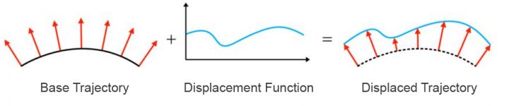
Mathematically, this process can be described as follows:


Both the choice of a base trajectory function, B(t), and a displacement function, D(t), will be the topics of the chapters to come and we will look at several interesting options to consider. In all cases, keep in mind the above expression for f(t) as it shows the most general and intuitive form of what we will be doing.
2 Modelling Lines and Curves
A path can be mathematically represented as a curve or line in space, and usually one has to choose between using some variation of an implicit curve model or a parametric curve model. We will be using parametric models entirely, with the parameter t usually in the range [0;1] and covering the path from start to finish. Still, it is worth to briefly discuss the differences between the two model classes and the reasons for choosing the parametric approach over the implicit one.


Looking at the linear path equations above, you might recognize the following two properties. First, if you are asked to determine if a random point in the scene belongs to the path, you are best off using the implicit form. Only points that belong to the line will result in upholding the two sides of the equation equal. Second, if you are asked to precisely trace the described path, one point after another, you are best off using the parametric form. Moving along a parameterized path requires simply advancing the value of the single parameter in the equation (t). In general, implicit forms represent tests/conditions for belonging to a given set and find applications in areas like collision detection and implicit geometric models for ray traced rendering; while parametric forms give a direct way to traverse a given set of points and find use in cases like shooting rays, drawing splines, and even performing interpolation.

(Comment: The above is an alternative implicit equation for a line in 2D. Note, that in 3D the equation no longer describes a line, but a plane, with normal N)
As noted above, we will be using parametric models. Another side advantage of parametric forms is that they do not depend on the dimensionality of the space, in which you are working. A parametric line connecting two points in space has the exact same form regardless of whether these points are in 2D, 3D, or any other dimension for that matter. Because of this, we will be able to do most of our work in 2D and then easily apply these results to 3D scenes.
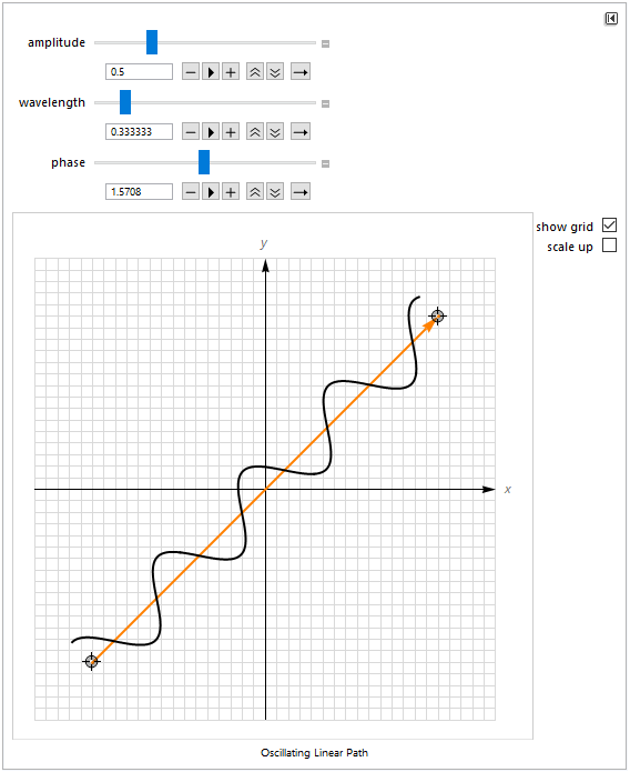
3 Modelling Oscillations
To model the planar oscillations for our fuzzy trajectories we chose to start with simple sine functions. The wave parameters that we exposed to our game designers included an amplitude (A), a wavelength (Lambda), and a phase (phi). An angular frequency can also be easily computed as (ⲱ = 1/Lambda).

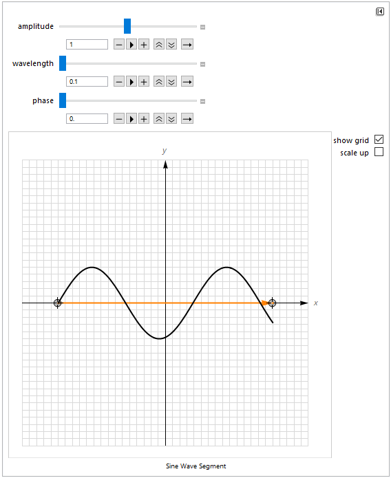
We next introduced a few simple, but very useful modifications to the starting sine model.
First of all, we had to make sure that for paths that are short relative to the desired oscillation amplitude we would proportionally diminish the fuzziness effect. This is needed so that for closer shots the projectile would not start its course in a weird direction, but instead would go towards the target more directly. To achieve this effect, we multiplied the amplitude by a factor of:

Second, we had to rescale the parameter t to the actual length of the path in world space. The result is that the distance to the target does not affect the observed frequency of oscillations, as it is now defined in world space:

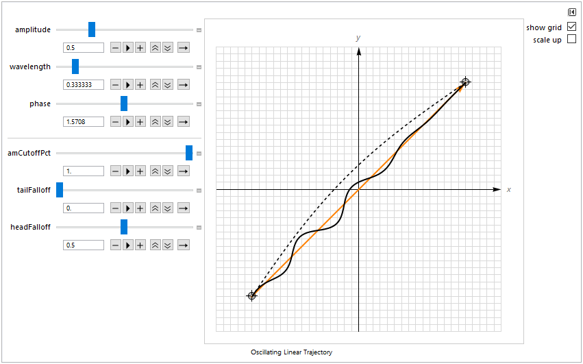
Third, we wanted to give our designers control over how fuzzy a trajectory would be at its beginning and ending. This allowed us to make projectiles that either start off more straight, before beginning to wobble, or, inversely, disperse initially, but end their trajectory with a sharper, precise hit. The latter option can be used to create the effect of the projectile having locked onto the target in midflight; while the former looks a bit more natural, as most people would find it strange if, because of fuzziness, the projectile were to leave the muzzle in some direction that is way off-target. Both path corrections were achieved simultaneity using amplitude falloffs:

One last amplitude modification, which we found useful, was the addition of a clamped sinusoidal scale factor, which further smoothed the start and end of the trajectory. The clamping factor was exposed to the designers as an amplitude cutoff percentage parameter:

Taking all of the above modifications into account, we can write the final fuzzy linear trajectory model as:


We kept the phase parameter (phi), as we found it to be useful for creating more diverse trajectories. As concrete examples, the parameter could be set at random for every fired shot, or could be made to vary for each projectile simultaneously fired by a multi-muzzle unit.
Also, note that we add the oscillation as a displacement in the orthogonal direction of the linear trajectory path. Expressed in this way, the equation holds both in 2D and 3D. For the 2D case, we obtain the normal direction by applying a 90Degree counter-clockwise rotation to the tangent vector. In 3D, a choice has to be made depending on the desired effect. For top-down games, it may be best to apply the fuzziness effect in a plane parallel to the ground. In other cases (e.g., view aligned effects, or 3D shooter scenes), other choices can be meaningful, too.
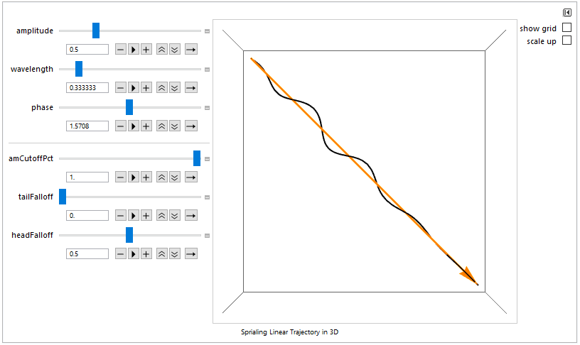
4 Modelling Swirls
As was described in the previous section, adding oscillations to our trajectories simply meant adding modified sinusoidal displacements along a chosen normal direction, perpendicular to the line towards the target. Swirls can be implemented in an almost identical manner, but we also need to choose a binormal displacement direction in addition to the tangent and normal vectors. Since our base path is linear, it is simplest to use our known forward direction vector and our previously chosen normal vector and construct the binormal as:

While one could experiment with all kinds of spirals and radial functions, we chose to implement our swirls using a simple helix. This choice naturally extends the sine functions from our oscillation models and thus provides the exact same parameters for our game designers to tweak.

The final model looks like this:


Note, that we preserved the same modifiers that allowed for extra control over the beginning and ending sections of the trajectory as well as the handling of short paths as in our oscillation model.
In-Game Examples
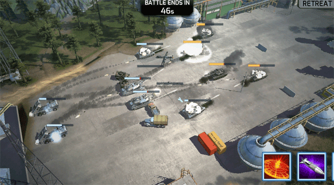
The footage below is from a prototype scene from the time that we first began to experiment with ballistic and fuzzy projectile paths.
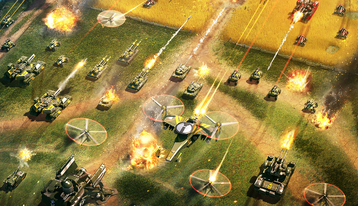
You may notice the resemblance between this scene and the battle scenes in WPO. Both WPO and BBRT are games that use our fuzzy trajectories via a C++ implementations of the models described in the previous section.
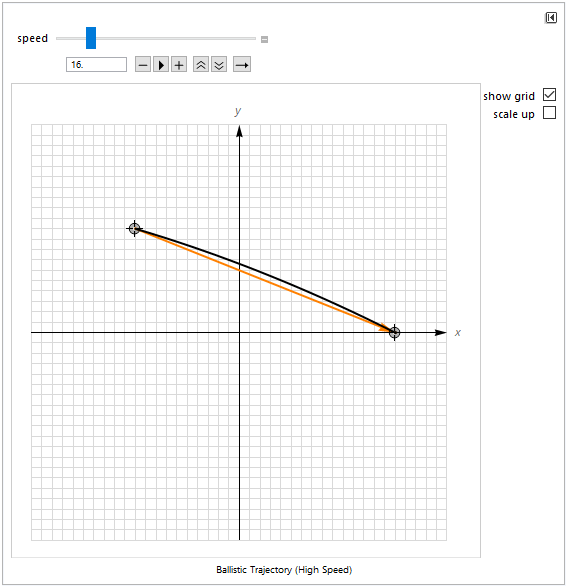
WPO makes heavier and more noticeable use of fuzzy trajectory projectiles, compared to BBRT. At present, both games use linear fuzzy paths only. Nevertheless, in a lot of cases linear base paths simply do not look natural. True projectile trajectories are parabolic and may be approximated by linear paths only for very high-speed projectiles. Because of this, we did implement a ballistic variant of the fuzzy paths, which I will describe in the last section of this article. Still, this model was used only in prototypes, since in some common cases that we faced going for physical accuracy was too restrictive for the game designers.
Specifically in the case of WPO, a transition to turn-based battle mechanics made the use of true ballistics impractical. It turned out that it was more important to be able to guarantee that each turn of fired shots can be completed within a very strict timeframe - with all projectiles having hit their targets. Increasing projectile speeds could solve the problem of hitting targets on time, but ends up changing the parabolic paths to ones that look more linear anyway. Here the best solution is to go for a model that is less physically accurate, but still physically plausible. As we will discuss in the next section, adding our fuzzy displacements to a quadratic Bézier curve is just the trick that we need in such cases. In reality, we have not had the time to revisit this problem in the context of WPO, but the fuzzy spline path functionality could be added to the game with some future updates.
Fuzzy Splines
As noted above, using linear segments as the base of our trajectories works only for relatively fast moving projectiles or very short travel distances. For most other cases, the base of the projectile path would have to be curved, because of the pull of gravity. Again, we would prefer the chosen curve model to be parametric, in order to fit as a base for our fuzzy displacements. Splines meet our requirements very well. There are different kinds of splines, depending on which of the spline control points the final curve passes through and how much control there is over the tangents and derivatives of the curve. For the purposes of modelling a projectile’s trajectory, we need a curve that passes exactly through some desired starting and ending points and leaves our firing muzzle at some desired angle. With these requirements in mind, it makes most sense to use Bézier curves, and even the simplest, quadratic version can suffice.
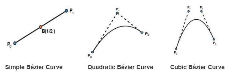
Coincidently, a true ballistic path is also described by a quadratic equation - a parabola. I will discuss this topic further in the next section, but, for now, it is good to know that we can obtain a physically plausible trajectory by using quadratic Bézier curves. The parametric formula for such a base curve is given by:

[Note: The above formula is simply the result of iterative application of linear interpolation, with every step of the iteration adding one more degree to the resulting curve.]
Before we can apply our fuzzy displacements to the spline model, we need to obtain a tangent, normal, and binormal vector for the trajectory. Those who are interested in doing something more advanced can look into obtaining a Frenet frame. For our purposes, we are going to use the same techniques and conventions described in the Modelling Swirls subsection above, which give us:


With a TBN frame at hand, applying fuzziness to a Bézier curve can be done by adding the following displacements to a Bézier base model:


For the length of the path, we used the linear distance between the starting and ending points. This is a simplification, which is fine for our needs. If you need extra precision on this, consider using some more advanced method for obtaining an arc length for a Bézier curve. Even using several linear segments to approximate the travelled path could suffice. In our case, will effectively are using just one such segment.
The resulting final formulas allow us to apply our fuzzy paths model to a new range of projectiles - ones with high-arcing trajectories. These include shots fired from cannons, howitzers, grenade launchers, mortars, and the like.
Fuzzy Ballistic Trajectories
 |
 |
 |
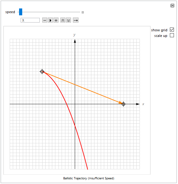
As was established in the previous section, with the use of quadratic Bézier curves one can get physically plausible results. Still, in some common cases it may be desirable to compute a true ballistic trajectory. Using the standard equations of motion and assuming an initial velocity (v0), no air drag or friction, and constant acceleration, we can come to the following position function:
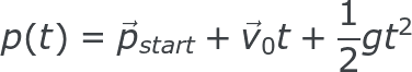
Here the magnitude of gravity is g ~= 9.8m/s^2, and later we will also use g-vector and g-hat to represent the directed and unit-length vectors for gravity, respectively. The expressed position function already is in parametric form, which is what we need. We specify a starting point (pstart) and a velocity vector (v0) and can express the path parameterized with respect to time, t.
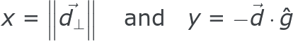
Still, for most of our use cases, we needed a different parameterization – one that more naturally extends our linear trajectories, which take as input a starting and ending point for the path. Therefore, we decided to solve for the initial launch angle based on the desired target location and the available projectile speed:

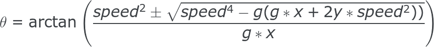
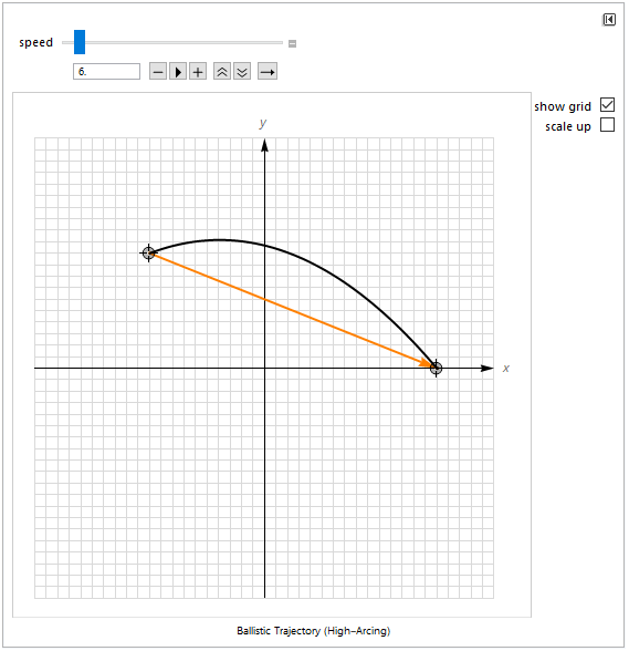
If the speed of the projectile is not high enough relative to the distance to the target, the solutions for theta are imaginary, and thus no real launch angle can result in a trajectory that hits the target. In cases like that, it may be best either to not shoot at all, or to launch the projectile at a 45° angle - guaranteeing maximum range, despite coming short of the target. On the other hand, when real valued solutions exist, you will have a choice between two possible shot angles. In most cases, it will make more sense to chose the smaller of the two solutions (using the ‘-’ sign when computing theta). This gives the more direct path. A caveat with this choice might be that the resulting path could become more straight than you want at higher launch speeds. Alternatively, you can solve for the high-arcing launch angle that gives a less direct path.
Having computed the launch angle, theta, we are ready to calculate the initial velocity as well as the time at which the trajectory will hit the target point:


The parametric base for our ballistic models, with a parameter t in the standard range [0;1], can now be expressed using the computed initial velocity and flight time:

To get to the final fuzzy ballistic trajectory model, we have to choose a TBN triplet. Doing this is no different than with the previous cases that we discussed, see the Fuzzy Splines section for more details. The final models can be written as:


For more details on implementing ballistic trajectories you can refer to this article. As was discussed in the previous section, if you want to have full control over the arcing of the path you can consider less physically accurate solutions.
Conclusion
The article showed that adding fuzzy displacements to a parametric base model for a path or trajectory can be done in a fairly straightforward and generic way. Two specific displacement functions were presented as examples - customized sinusoids and helixes. Both give a simple set of parameters, which can be used by game designers to achieve a wide variety of curve behaviours. While these fuzziness models can be applied to any parametric base function, the ones that have been found to be of particularly practical use include: linear base paths; true ballistic paths; and spline-based curved paths.
Several of these models have already been used in some of Gameloft’s titles. In particular, War Planet Online: Global Conquest (WPO) and Blitz Brigade: Rival Tactics (BBRT) make use of fuzzy projectiles in their battle scenes. While all current use cases for our fuzzy paths have been battle related, the same models can be used in many other contexts. The first that comes to mind is hair simulation, where each hair filament is a fuzzy curve. Fluid flow is another context where fuzzy curves can find application.